Image segmentation is a branch of computer vision which aims to provides a human oriented interpretation of an image. We humans are able to visualize the contours/boundaries of objects in an image which allows us to distinguish the particular object from the rest of the scene. However to a computer an object is just a representation of some individual pixel values without any context. Image segmentation attempts to partition the image into segments (representing individual objects) that are more meaningful and easier to analyze. More technically, image segmentation is a process of assigning labels to individual pixels in the image such that the pixels with similar characteristics share the same label.
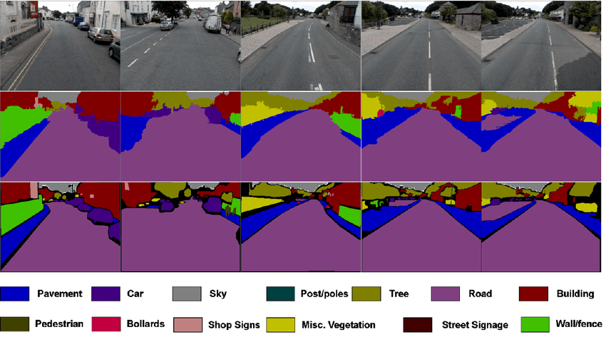
Semantic segmentation of street level data (middle row) followed by CRF model (bottom row) (Image Credit: Sunando Sengupta, et. al., 2012 )
Presently image segmentation is being popularly used in medical imaging, remote sensing and self-driving cars. This is because image segmentation makes it easier for an intelligent system to make decisions based on meaningful objects in the scene rather than individual pixels. If you are not familiar with segmentation, then stay tuned as this post will help you gain a quick understanding of some of the most popular segmentation architectures.
Seeded Region Growing
Seeded Region Growing (SRG) is one of the most popular segmentation architectures that has been widely used in medical imaging and remote sensing. There are two main ideas behind SRG: i) identify the approximate location of the objects in the scene (known as seeds) ii) grow the seeds into regions that identify the object in the image. Using some multi-spectral LiDAR data (courtesy of Optech. Inc) I ran a modified variant of SRG to delineate individual tree crowns. Below are the seed selection and SRG results for a patch from the original LiDAR scan.


Initial seeds (left) Contours of the grown regions (right)
I will not discuss seed selection here as that is a whole new topic but generally seed selection methods depend on the nature of objects we are trying to segment in the image (i.e. for medical imaging and remote sensing morphological based operations, and local maxima/minima detectors are commonly used). The initial seeds are used as approximate location of the objects in the image. Using these seeds the connecting neighboring pixels (4-connected or 8-connected) are examined to check if they are similar to the seed. First and second order statistics (mean and variance) are commonly used for computing similarity metrics and hence it helps to have the initial seeds as at least few pixels so that the computed statistics are meaningful. Usually the vanilla version of SRG is modified with additional constraints (shape based constraints, energy minimization constraints, region compactness constraints and et cetera) to make it more suitable for the desired application. To give an example, the variant of SRG that I implemented had a shape constraint to ensure that the grown regions did not have a long tail. Since I was dealing with structural and spectral data I had additional structural constraints to ensure that the grown regions were constrained by a Gaussian structure (this is because I was trying to segment tree crowns). SRG is a relatively straightforward algorithm but with the addition of different constraints it can become complicated and slow.
Many people confuse SRG with region growing which is a different method. In region growing, we do not rely on prior seed selection; instead each individual pixel is viewed as an individual seed and the method tries to merge neighboring pixels based on their similarity to each other. Since there are no prior approximations of the objects present in the image, the method is not as accurate as SRG and hence is not commonly used.
Marker Controlled Watershed
Marked Controlled Watershed (MCW) is another popular segmentation algorithm that relies on an underlying mathematical morphology in the scene to segment individual objects. In MCW the image is viewed as an inverted topological surface with pits as the local minima (formally known as catchment basins) and the boundary between objects as the local maxima (watershed lines). The idea behind the algorithm is that of a flood-fill based approach. A set of markers, pixels where the flooding starts, are initially selected like in SRG. The neighboring pixels of the markers are examined and stored in the order of their gradient magnitude. Then starting from the pixel with the lowest gradient magnitude we extract its neighbor to check if they all have the same labels. We label the pixel with same label as its neighbors if all the neighbors share a common label. The unlabeled pixels are then the watershed lines that represent the contours of the objects and the labelled pixels represent the segmented objects.


Initial Markers (left) Result of MCW segmentation (right)
In implementation of MCW priority queues are commonly used to store the pixels as their gradient magnitude can be used as indicator for the priority of extraction. Different variants of MCW have been proposed since Meyer’s flooding algorithm in the 90s. However one of the key problems that I have encountered with MCW, as compared to SRG, is that it is much more difficult to incorporate constraints in the implementation. In SRG we do not assume an underlying physical structure in the image, but in MCW the image is viewed as a topological surface. The assumed structure in the image makes it more difficult for additional constraints to be implemented. Also MCW does not work well with scenes where the topological structure cannot be assumed (i.e. segmenting individual trees in a multispectral image or medical imaging).
Fully Convolutional Networks
So far we have talked about the two most popular traditional segmentation methods that date back to the 80s (pretty old eh!). While these traditional segmentation methods are still popularly used today, we have seen the growth of deep learning architectures in performing instance segmentation. A paper from UC Berkeley introduced Fully Convolutional Networks that could learn to make dense predictions on per pixel level basis for segmentation tasks. The proposed architecture is much simpler than its competitor (Mask-RCNN) which requires rather extensive proposal generations. The FCN architecture relies on end-to-end convolutional layers to learn pixel-wise predictions. The structure of the network is based upon encoder-decoder architecture, where the initial 7 layers of the network are layers of a typical CNN, and subsequent layers are used for generating the segmentation map by up sampling the results. In the FCN structure the fully connected layer (7th layer) is replaced by a 1×1 convolutional layer which generates a heatmap of the features detected by network. This network architecture is popularly dubbed as pixel-to-pixel architecture, as the labels are pixelwise predictions of the same 2D dimensions as the input image.
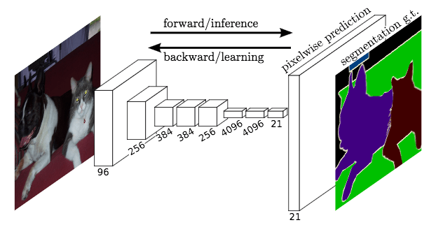
Structure of FCN (Image Credit: Long, et. al., 2015)
The output from the network is up sampled using deconvolutional operations. Since the up sampled images are coarse, the FCN architecture makes use of the feature maps from earlier layers to refine the coarse segmentation. These additions are known as skip connections.
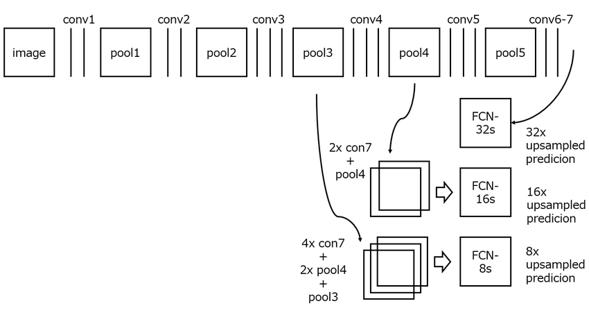
Skip Connections in FCN (Image Credit: Long, et. al., 2015)
In the original paper the authors present three different examples of the FCN architecture: FCN-32, FCN-16 and FCN-8. FCN-32 directly produces segmentation maps from the 7th convolution layer by using a deconvolution operation with a stride of 32 pixels. This results in a 32x up sampling from the output of the final convolution layer, hence yielding the same 2D dimensions as the input image. Since no skip connections are applied from previous layers, the segmentation results are coarse. FCN-16 and FCN-8 are 16x and 8x up sampling of the output, respectively. In FCN-16 the output of the final 1×1 convolutional layer are up sampled by 16x and the activations from pooling layer 4 are added. This results in a relatively refined segmentation result. In FCN-8, outputs from further pooling layer 3 are added to the results which further helps retrieve fine-grained spatial information.
Unfortunately, I did not have enough training data to run the FCN for this particular dataset, but I will make another post with a road crack detection dataset that I am presently working on.
Bonus (Edge detectors)!
I have included edge detection here, even though it is not formally regarded as a segmentation method. However, edge detection, combined with edge connectivity, has been frequently used for segmenting images. This is because while edge detection methods do not yield closed regions like SRG, MCW or FCN, they can identify the contours (i.e. edges) of the objects. To further close the regions, edge connectivity (or linking) is used to connect the edge pixels. Although the results are not comparable to MCW or SRG, the major edges between objects can still be identified.

Canny edge detection
For the LiDAR data, Canny edge detector was able to pick up the major contours however it could not distinguish between the tree clusters (which is one of the main goals of individual tree crown identification). This is one of the major setbacks of edge detection methods when used for segmentation purposes.
So now that you are hopefully somewhat familiar with segmentation, you can code up your examples. OpenCV is a great start but do not rely on it too much as it only provides the vanilla versions these methods. If you are interested in my implementation of SRG, you can find my paper here.
